Definition 4.7.1 Weighted Graphs
A weighted graph is a graph with numbers assigned to each edge. The assigned numbers are the edge weights of the graph.
In this section we will see an algorithm to find the shortest path between two vertices in a weighted graph.
Sometime it makes sense to assign a weight to each edge of a graph. The weights might represent distances between cities, travel times, or costs.
A weighted graph is a graph with numbers assigned to each edge. The assigned numbers are the edge weights of the graph.
The graph below is a weighted graph.
When you visit a website like Google Maps or use your Smartphone to ask for directions from home to your Aunt’s house in Pasadena, you are usually looking for a shortest path between the two locations. These computer applications use representations of the street maps as graphs, with estimated driving times as edge weights.
While often it is possible to find a shortest path on a small graph by guess-and-check, our goal in this chapter is to develop methods to solve complex problems in a systematic way by following algorithms. An algorithm is a step-by-step procedure for solving a problem. Dijkstra’s (pronounced dike-stra) algorithm will find the shortest path between two vertices.
Mark the ending vertex with a distance of zero. Designate this vertex as current.
Find all vertices leading to the current vertex. Calculate their distances to the end. Since we already know the distance the current vertex is from the end, this will just require adding the most recent edge. Don’t record this distance if it is longer than a previously recorded distance.
Mark the current vertex as visited. We will never look at this vertex again.
Mark the vertex with the smallest distance as current, and repeat from step 2.
Suppose you need to travel from Tacoma, WA (vertex T) to Yakima, WA (vertex Y). Looking at a map, it looks like driving through Auburn (A) then Mount Rainier (MR) might be shortest, but it’s not totally clear since that road is probably slower than taking the major highway through North Bend (NB). A graph with travel times in minutes is shown below. An alternate route through Eatonville (E) and Packwood (P) is also shown.

Step 1: Mark the ending vertex with a distance of zero. The distances will be recorded in [brackets] after the vertex name.
Step 2: For each vertex leading to Y, we calculate the distance to the end. For example, NB is a distance of 104 from the end, and MR is 96 from the end. Remember that distances in this case refer to the travel time in minutes.

Step 3 & 4: We mark Y as visited, and mark the vertex with the smallest recorded distance as current. At this point, P will be designated current. Back to step 2.
Step 2 (#2): For each vertex leading to P (and not leading to a visited vertex) we find the distance from the end. Since E is 96 minutes from P, and we’ve already calculated P is 76 minutes from Y, we can compute that E is 96+76 = 172 minutes from Y.

If we make the same computation for MR, we’d calculate 76+27 = 103. Since this is larger than the previously recorded distance from Y to MR, we will not replace it.
Step 3 & 4 (#2): We mark P as visited, and designate the vertex with the smallest recorded distance as current: MR. Back to step 2.
Step 2 (#3): For each vertex leading to MR (and not leading to a visited vertex) we find the distance to the end. The only vertex to be considered is A, since we’ve already visited Y and P. Adding MR’s distance 96 to the length from A to MR gives the distance 96+79 = 175 minutes from A to Y.

Step 3 & 4 (#3): We mark MR as visited, and designate the vertex with smallest recorded distance as current: NB. Back to step 2.

Step 2 (#4): For each vertex leading to NB, we find the distance to the end. We know the shortest distance from NB to Y is 104 and the distance from A to NB is 36, so the distance from A to Y through NB is 104+36 = 140. Since this distance is shorter than the previously calculated distance from Y to A through MR, we replace it.
Step 3 & 4 (#4): We mark NB as visited, and designate A as current, since it now has the shortest distance.
Step 2 (#5): T is the only non-visited vertex leading to A, so we calculate the distance from T to Y through A: 20+140 = 160 minutes.
Step 3 & 4 (#5): We mark A as visited, and designate E as current.
Step 2 (#6): The only non-visited vertex leading to E is T. Calculating the distance from T to Y through E, we compute 172+57 = 229 minutes. Since this is longer than the existing marked time, we do not replace it.
Step 3 (#6): We mark E as visited. Since all vertices have been visited, we are done.
From this, we know that the shortest path from Tacoma to Yakima will take 160 minutes. Tracking which sequence of edges yielded 160 minutes, we see the shortest path is T-A-NB-Y.
Dijkstra’s algorithm is an optimal algorithm, meaning that it always produces the actual shortest path, not just a path that is pretty short, provided one exists. This algorithm is also efficient, meaning that it can be implemented in a reasonable amount of time. Dijkstra’s algorithm takes around \(V^2\) calculations, where \(V\) is the number of vertices in the graph. A graph with 100 vertices would take around 10,000 calculations. While that would be a lot to do by hand, it is not a lot for computer to handle. It is because of this efficiency that your car’s GPS unit can compute driving directions in only a few seconds.
In contrast, an inefficient algorithm might try to list all possible paths then compute the length of each path. Trying to list all possible paths could easily take \(10^{25}\) calculations to compute the shortest path with only 25 vertices; that’s a 1 with 25 zeros after it! To put that in perspective, the fastest computer in the world would still spend over 1000 years analyzing all those paths.
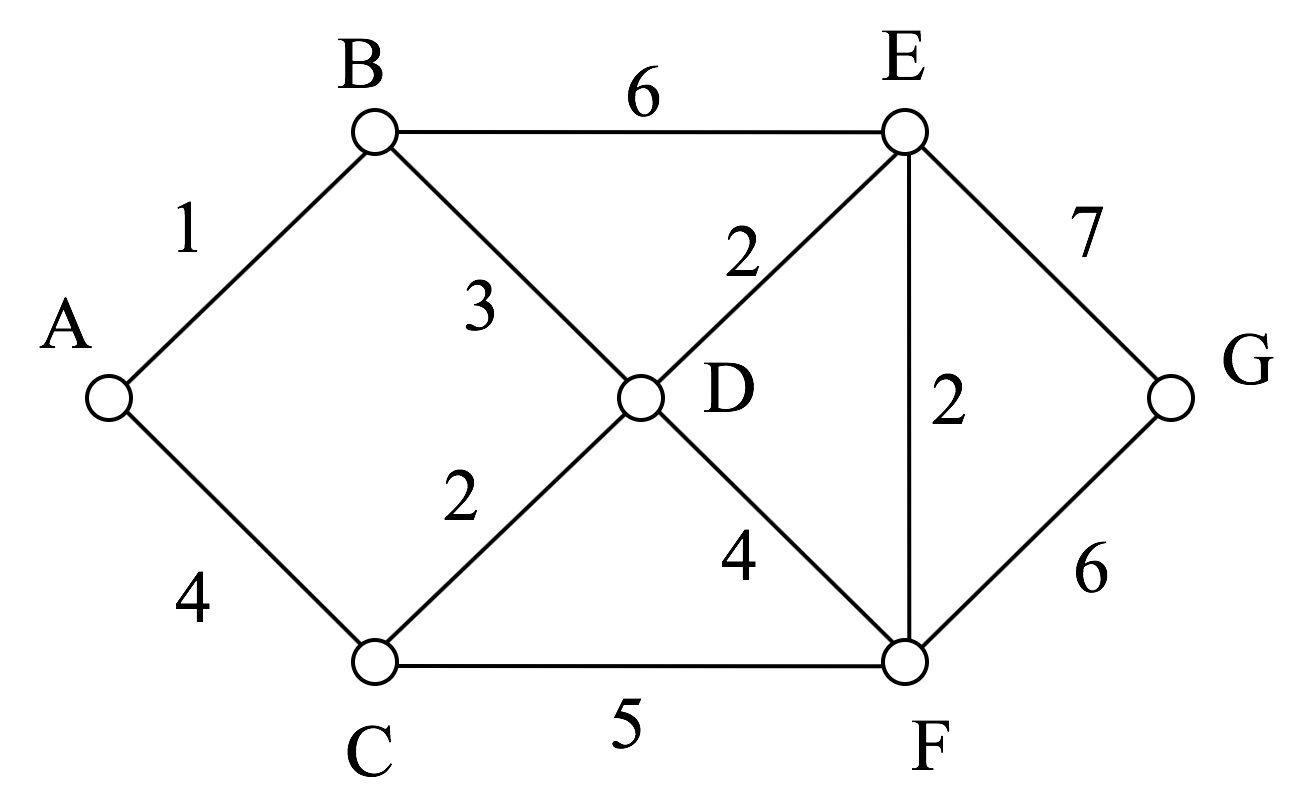
Find the shortest path between vertices A and G in the graph below.
The table below shows approximate driving times (in minutes, without traffic) between five cities in the Dallas area. Create a weighted graph representing this data.
| Plano | Mesquite | Arlington | Denton | |
| Fort Worth | 54 | 52 | 19 | 42 |
| Plano | 38 | 53 | 41 | |
| Mesquite | 43 | 56 | ||
| Arlington | 50 |
Travel times by rail for a segment of the Eurail system is shown below with travel times in hours and minutes . Find path with shortest travel time from Bern to Berlin by applying Dijkstra’s algorithm.

Using the graph from the previous problem, find the path with shortest travel time from Paris to München.